Understanding Gradients in Machine Learning by Implementing Numerical Differentiation and Gradient Checking From Scratch¶

When we train machine learning models using frameworks like PyTorch, TensorFlow, or JAX, we rely heavily on automatic differentiation.

These frameworks magically compute gradients for us.

But something bothered me while learning machine learning:

I was using gradients every day but didn't truly understand what was happening under the hood.

So I decided to implement the core ideas myself.

The goal of this project was to deeply understand:

Numerical differentiation
Gradients of multivariable functions
Gradient checking
Linear regression gradients
Neural network gradients

This project forced me to connect calculus, optimization, and machine learning in a practical way.

Why Gradients Matter in Machine Learning¶

Nearly every machine learning model is trained using Gradient Descent.

The goal of training is simple:

We want to minimize a loss function.

\[ L(\theta) \]

Where:

\(L\) = loss
\(\theta\) = model parameters

Training updates parameters using the gradient:

\[ \theta_{new} = \theta - \alpha \nabla L(\theta) \]

Where:

\(\alpha\) = learning rate
\(\nabla L(\theta)\) = gradient of the loss

Intuitively:

Think of the loss function as a landscape of hills and valleys.

The gradient tells us:

Which direction is downhill?

Visualizing Optimization¶

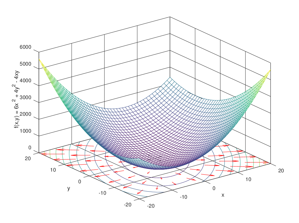
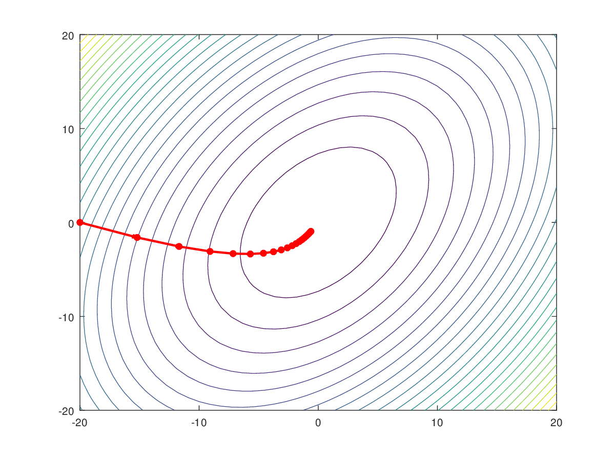
In the figures above:

The surface represents the loss function.
The red path shows the steps taken by gradient descent.
Eventually the algorithm reaches the minimum.

This idea powers training in everything from:

linear regression
neural networks
deep learning models

Part 1 — Understanding Derivatives Numerically¶

Before working with gradients, we need to understand derivatives.

The derivative measures how fast a function changes.

Mathematically:

\[ f'(x) = \lim_{h \to 0} \frac{f(x+h) - f(x)}{h} \]

This definition means:

The derivative is the slope of the tangent line.

But computers cannot evaluate limits.

Instead we approximate derivatives using finite differences. ([m3lab.github.io][1])

Forward, Backward, and Central Difference¶

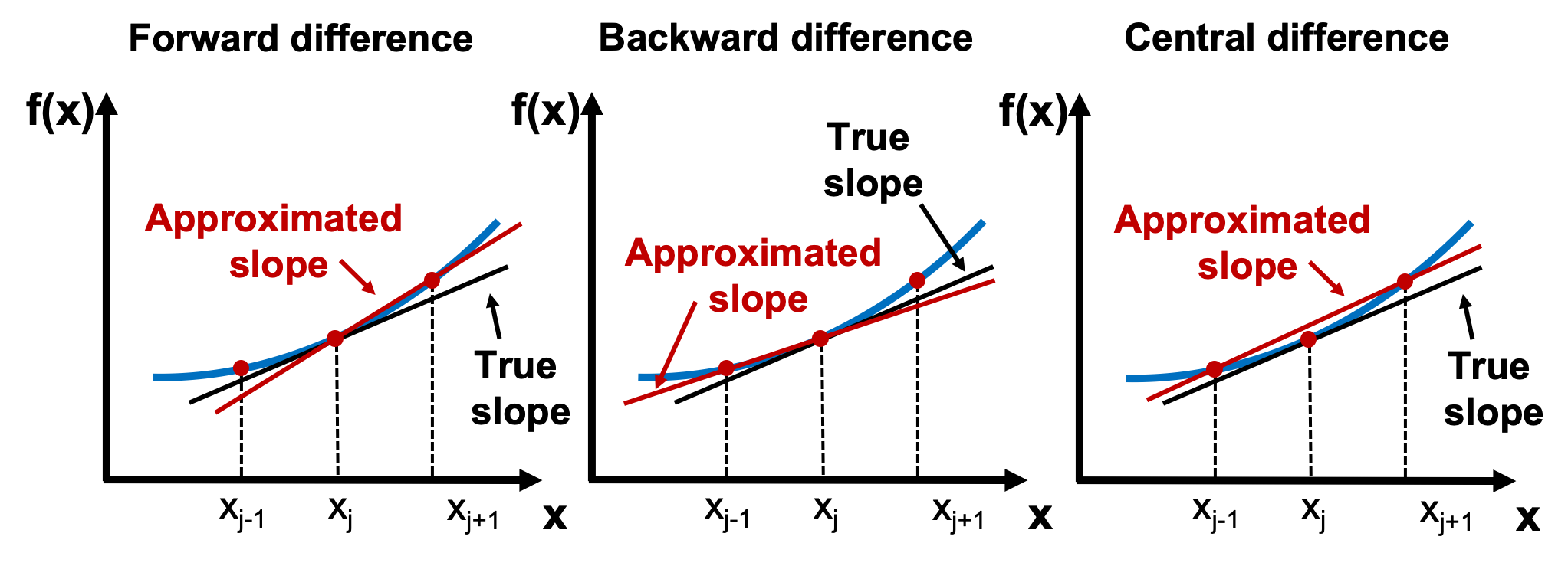
Finite difference methods approximate derivatives using nearby points.

Forward Difference¶

\[ f'(x) \approx \frac{f(x+h)-f(x)}{h} \]

Python implementation:

def forward_difference_derivative(f, x, h=1e-6):
    return (f(x + h) - f(x)) / h

Interpretation:

We estimate the slope by looking slightly ahead of x.

Backward Difference¶

\[ f'(x) \approx \frac{f(x)-f(x-h)}{h} \]

Implementation:

def backward_difference_derivative(f, x, h=1e-6):
    return (f(x) - f(x - h)) / h

Here we estimate the slope using the point just behind x.

Central Difference (Best Approximation)¶

\[ f'(x) \approx \frac{f(x+h)-f(x-h)}{2h} \]

Implementation:

def central_difference_derivative(f, x, h=1e-6):
    return (f(x + h) - f(x - h)) / (2 * h)

This method is usually more accurate because it considers both sides of the point. ([uclnatsci.github.io][2])

Testing the Methods¶

I tested these numerical derivatives on known functions.

Example:

\[ f(x) = x^2 \]

Derivative:

\[ f'(x) = 2x \]

At (x = 3):

\[ f'(3) = 6 \]

When we compute the numerical derivative, we get values extremely close to 6.

Symbolic Derivatives¶

To verify correctness, I also used SymPy.

This library computes exact derivatives symbolically.

Example:

from sympy import Symbol, sympify, diff

def symbolic_derivative(expr, var="x"):
    x = Symbol(var)
    sym_expr = sympify(expr)
    return diff(sym_expr, x)

Example result:

symbolic_derivative("x**2")

returns

2*x

Part 2 — Gradients of Multivariable Functions¶

Machine learning models usually depend on many variables.

Example function:

\[ f(x,y)=x^2+y^2 \]

The gradient is defined as:

\[ \nabla f = \begin{bmatrix} \frac{\partial f}{\partial x} \\ \frac{\partial f}{\partial y} \end{bmatrix} \]

Which equals:

\[ \nabla f = \begin{bmatrix} 2x \\ 2y \end{bmatrix} \]

Gradient Visualization¶

Each arrow represents the direction of steepest increase.

Key idea:

The gradient always points uphill.

To minimize loss, we move in the opposite direction.

Implementing Numerical Gradient¶

To compute gradients numerically, we slightly perturb each parameter.

Implementation:

def numerical_gradient(f, params, h=1e-6):
    grad = [0.0] * len(params)

    for i in range(len(params)):
        original = params[i]

        params[i] = original + h
        f_plus = f(params)

        params[i] = original - h
        f_minus = f(params)

        grad[i] = (f_plus - f_minus) / (2 * h)

        params[i] = original

    return grad

This works for any function, regardless of complexity.

Part 3 — Gradient Checking¶

When implementing machine learning algorithms manually, it is very easy to make mistakes.

Gradient checking helps verify correctness.

Steps:

Compute analytical gradient
Compute numerical gradient
Compare them

Relative Error Formula¶

To compare gradients we compute:

\[ \text{Relative Error} = \frac{|g_{analytic}-g_{numeric}|} {\max(|g_{analytic}|,|g_{numeric}|)} \]

If the error is small (e.g. (10^{-6})), the gradients match.

Implementation:

rel_error = abs(ga - gn) / max(abs(ga), abs(gn), 1e-12)

Part 4 — Linear Regression Gradient¶

Linear regression model:

\[ y = wx + b \]

Loss function: Mean Squared Error

\[ L = \frac{1}{N}\sum (wx + b - y)^2 \]

Analytical Gradients¶

Weight gradient:

\[ \frac{\partial L}{\partial w} = \frac{2}{N}\sum (wx + b - y)x \]

Bias gradient:

\[ \frac{\partial L}{\partial b} = \frac{2}{N}\sum (wx + b - y) \]

I implemented this directly in Python.

Gradient checking confirms that the analytical and numerical gradients match.

Part 5 — Neural Network Gradient¶

Finally, I applied gradient checking to a tiny neural network.

Architecture:

Input → Linear Layer → Sigmoid → Binary Cross Entropy Loss

Sigmoid Function¶

\[ \sigma(z) = \frac{1}{1+e^{-z}} \]

It converts any real number into a value between 0 and 1.

This makes it useful for binary classification.

Binary Cross Entropy Loss¶

\[ L = -[y\log(a) + (1-y)\log(1-a)] \]

Where:

\(y\) = true label
\(a\) = predicted probability

Key Derivative Result¶

For sigmoid + BCE, the derivative simplifies to:

\[ \frac{\partial L}{\partial z} = a - y \]

This simplification is what makes neural network training efficient.

Neural Network Gradient¶

Using the chain rule:

\[ dw = \frac{1}{N}\sum (a-y)x \]

\[ db = \frac{1}{N}\sum (a-y) \]

I implemented these gradients and verified them using gradient checking.

Why Gradient Checking Is Important¶

Even large organizations like:

OpenAI
Google DeepMind
Meta AI

use gradient checking when developing new architectures.

Why?

Because even a small derivative mistake can completely break training.

What I Learned From This Project¶

Implementing everything manually helped me understand:

• Why gradients work • How optimization works mathematically • Why numerical gradients are useful for debugging • How neural network training really works

Instead of treating machine learning frameworks as black boxes, I now understand what is happening under the hood.

Final Thoughts¶

This project connected several fundamental concepts:

Calculus
Optimization
Machine learning

Understanding these from first principles made the entire ML training process much clearer.

If you're learning machine learning, I strongly recommend implementing these ideas from scratch at least once.

It completely changes how you think about training models.